Generalized Drift Diffusion Model diagram

Summary

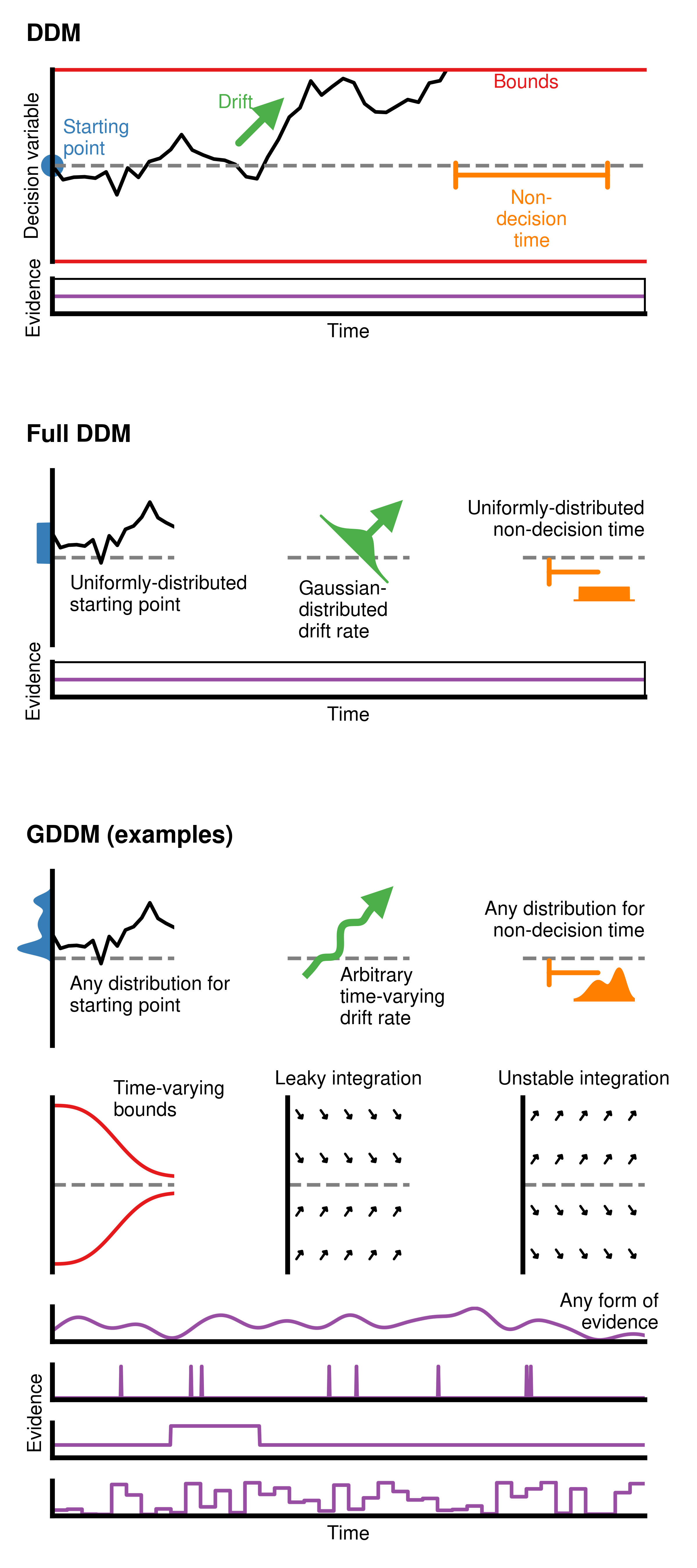
Here, we will show how to build each individual component found in the diagram describing the generalized drift diffusion model (GDDM), as seen in Figure 1 from Shinn et al. 2020. This is a good demonstration because it does not require data files to produce.

Setting up the figure

First, we import the plotting libraries and define some basic properties:

from ddm import Model, DriftConstant
import matplotlib.pyplot as plt
import numpy as np
import seaborn as sns
import scipy.stats
import random

sns.set_palette("Set1")
color_bound = sns.color_palette()[0]
color_x0 = sns.color_palette()[1]
color_drift = sns.color_palette()[2]
color_ev = sns.color_palette()[3]
color_nd = sns.color_palette()[4]

Define a function we will use later to make the plotting look nice:

def set_up_plot(ax):
    sns.despine(bottom=True, ax=ax)
    ax.axhline(0, c="gray", linestyle="--")
    ax.set_xlim(0, 0.55)
    ax.set_ylim(-1, 1)
    ax.set_xticks([])
    ax.set_yticks([])
    ax.spines["left"].set_linewidth(2)

Now, we initialize the Canvas object within CanD:

from cand import Canvas, Width, Height, Point, Vector

c = Canvas(4, 9)
c.set_font("Nimbus sans", size=8)

DDM schematic

We create a new unit, which we call “absolute2”. We do this so that we can use a separate coordinate system for each part of the plot. This makes it easy to adjust the position of the different parts separately. Then, we set it as the default unit so that we don’t have to worry about adding “absolute2” to the end of all of our Points:

c.add_unit("absolute2", Vector(1, 1, "absolute"), Point(0, 1, "absolute"))
c.set_default_unit("absolute2")

We add two axes, one for the actual DDM, and one for the plot showing the change in evidence over time:

c.add_axis("ddm", Point(0.3, 6.5), Point(3.7, 7.6))
c.add_axis("evidence", Point(0.3, 6.2), Point(3.7, 6.4))

First, we simulate the model to create the diagram. Note that we make some cosmetic changes to the DDM trace for the purpose of clarity within the diagram:

model = Model(drift=DriftConstant(drift=0.8), dt=0.01, dx=0.01)
sim_trial = model.simulate_trial(seed=8)
sim_trial[20:] = -sim_trial[20:] * 1.6
sim_trial = sim_trial[0:38]

Next, we plot the trace on the axis, and draw the upper and lower bounds on the same axis:

ax = c.ax("ddm")
ax.plot(model.t_domain()[0 : len(sim_trial)], sim_trial, c="k")
ax.axhline(1, c=color_bound, clip_on=False)
ax.axhline(-1, c=color_bound, clip_on=False)
ax.set_ylabel("Decision variable")
set_up_plot(ax)

Now, we annotate the DDM diagram. First, we draw an an arrow to denote the non-decision time. We make the arrow a distance indicator, and change the shape to make it attractive. We position it using the non-decision time startpoint, determined from the coordinates within the axis:

non_decision_time = 0.15
ndstartpoint = Point(model.t_domain()[37], -0.1, "ddm")
c.add_arrow(
    ndstartpoint,
    ndstartpoint + Vector(non_decision_time, 0, "ddm"),
    arrowstyle="|-|,widthA=5,widthB=5",
    color=color_nd,
)
c.add_text(
    "Non-\ndecision\ntime",
    ndstartpoint + Vector(non_decision_time / 2, -0.15, "ddm"),
    verticalalignment="top",
    color=color_nd,
)
ndgap = 0.003

Label the bounds:

c.add_text("Bounds", Point(0.8, 0.93, "axis_ddm"), color=color_bound)

Draw an arrow indicating the drift rate, and label it:

arrow_start = Point(0.17, 0.2, "ddm")
arrow_len = Vector(0.3, 0.3, "absolute")
c.add_arrow(
    arrow_start,
    arrow_start + arrow_len,
    arrowstyle="-|>,head_width=4,head_length=8",
    lw=3,
    color=color_drift,
    joinstyle="miter",
)
c.add_text(
    "Drift",
    arrow_start + arrow_len.height(),
    verticalalignment="top",
    color=color_drift,
)

Draw and label the starting point:

ax.scatter([0], [0], color=color_x0, s=70, clip_on=False)
c.add_text(
    "Starting\npoint",
    Point(0.01, 0.07, "ddm"),
    horizontalalignment="left",
    verticalalignment="bottom",
    color=color_x0,
)

Draw and label the evidence over time:

ax = c.ax("evidence")
ax.plot([0, 1], [1, 1], c=color_ev)


def make_evgrid_axis(ax):
    ax.set_xticks([])
    ax.set_yticks([])
    ax.set_xlim([0, 1])
    ax.spines["left"].set_linewidth(2)
    ax.spines["bottom"].set_linewidth(2)


make_evgrid_axis(ax)
ax.set_xlabel("Time")
ax.set_ylabel("Evidence")

Full DDM schematic

First, we set up a grid of axes for the starting point, variable drift rate, and non-decision time features of the Full DDM, as well as the evidence over time axis:

c.add_grid(
    ["fullx0", "fulldrift", "fullnd"],
    1,
    Point(0.3, 4.3),
    Point(3.7, 5.3),
    size=Vector(0.7, 1),
)
c.add_axis("evidence_ddm", Point(0.3, 4.0), Point(3.7, 4.2))

The following will allow us to draw any distribution sideways on an axis. We write this as a function because, while it is simply a uniform distribution here, we will want to draw a more complicated distribution later for the GDDM. This functions by transforming the points to data space, setting the clip off, and then filling in the region between the curve and the axis. This is mostly performed in pure matplotlib, and does not require features from CanD:

def make_starting_position_plot(axname, dist_func):
    zoom_area = (-0.9, 0.9)
    ax = c.ax(axname)
    dist_x = np.linspace(zoom_area[0], zoom_area[1], 500)
    ax.fill_betweenx(
        dist_x, -(dist_func(dist_x)) / 70, 0, clip_on=False, color=color_x0
    )
    set_up_plot(ax)
    ax.set_ylim(*zoom_area)
    ax.set_xlim(0, 0.3)
    offset = 0.25
    ax.plot(model.t_domain()[0 : len(sim_trial)] * 2, offset + sim_trial, c="k")


make_starting_position_plot("fullx0", scipy.stats.uniform(-0.05, 0.4).pdf)
c.add_text(
    "Uniformly-distributed\nstarting point",
    Point(0, 0, "fullx0") + Vector(0.1, -0.1, "absolute"),
    horizontalalignment="left",
    verticalalignment="top",
)

We also draw an arbitrary distribution for the non-decision time. By contrast, this uses some features of CanD. It operates by creating a new axis on top of the existing axis, turning off the spines, and drawing the distribution on the new axis. Then, it uses CanD to draw an “arrow” (that looks like “|—“), similar to the one drawn on the DDM plot:

def make_ndtime(axname, dist_func, height=0.05):
    ax = c.ax(axname)
    set_up_plot(ax)
    ax.set_xlim(0, 0.3)
    ax.set_ylim(-0.3, 0.3)
    c.add_axis(
        axname + "dist",
        Point(0.05 + non_decision_time / 2, -0.15, axname),
        Point(0.05 + non_decision_time * 1.5, -0.15 + height, axname),
    )
    c.ax(axname + "dist").axis("off")
    nddist_x = np.linspace(-1, 1, 500)
    c.ax(axname + "dist").fill_between(
        nddist_x, dist_func(nddist_x) / 50, 0, color=color_nd
    )
    c.ax(axname + "dist").set_xlim(-1, 1)
    sns.despine(ax=ax, left=True, bottom=True)
    c.add_arrow(
        Point(0.05 + ndgap, -0.05, axname),
        Point(0.05 + non_decision_time - ndgap, -0.05, axname),
        arrowstyle="|-|,widthA=5,widthB=0",
        color=color_nd,
    )


make_ndtime("fullnd", scipy.stats.uniform(-0.8, 1.6).pdf)
c.add_text(
    "Uniformly-distributed\nnon-decision time",
    Point(1, 0.5, "axis_fullnd") + Vector(0, 0.1, "absolute"),
    horizontalalignment="right",
    verticalalignment="bottom",
)

Lastly, we draw the drift rate. We seek to draw an arrow with a Gaussian distribution at the bottom. We accomplish this by defining a Gaussian distribution, rotating it by 45 degrees, placing it on a new axis. We set the position of the new axis based on the position of the arrow:

ax = c.ax("fulldrift")
set_up_plot(ax)
arrgapx = 0.05
arrgapy = 0.05
anchor = 0.15
arrlen = Vector(0.3, 0.3, "absolute")
ax.set_ylim(-0.5, 0.5)
ax.set_xlim(anchor - 0.01, anchor + 0.1)
arrowtilt = Vector(0, 0)
arrow_lr = Point(anchor + arrgapx, arrgapy, "fulldrift")
c.add_arrow(
    arrow_lr,
    arrow_lr + arrlen + arrowtilt,
    arrowstyle="-|>,head_width=4,head_length=8",
    lw=3,
    color=color_drift,
    joinstyle="miter",
)
sns.despine(ax=ax, left=True, bottom=True)
drift_x = np.linspace(-1, 1, 500)
drift_mat = np.asarray([drift_x, scipy.stats.norm(0, 0.3).pdf(drift_x) / 3]).T
cos, sin = np.cos(3.141592 / 4), np.sin(3.141592 / 4)
rotated_drift_mat = drift_mat @ np.array([[cos, -sin], [sin, cos]])
c.add_axis("miniarrowdist", arrow_lr - arrlen * 0.7, arrow_lr + arrlen * 0.7)
c.ax("miniarrowdist").axis("off")
c.ax("miniarrowdist").fill_between(
    rotated_drift_mat[:, 0],
    rotated_drift_mat[:, 1],
    -rotated_drift_mat[:, 0],
    color=color_drift,
)
c.add_text(
    "Gaussian-\ndistributed\ndrift rate",
    Point(anchor, 0, "fulldrift") + Vector(0, -0.13, "absolute"),
    horizontalalignment="left",
    verticalalignment="top",
)

And, as before, we plot the constant evidence signal:

ax = c.ax("evidence_ddm")
ax.plot([0, 1], [1, 1], c=color_ev)
make_evgrid_axis(ax)
ax.set_xlabel("Time")
ax.set_ylabel("Evidence")

GDDM

First, we work on the six main plots showing GDDM features. We will look at the evidence streams later. As in the Full DDM case, create a grid of axes:

c.add_grid(
    ["gddmx0", "gddmdrift", "gddmnd", "gddmbounds", "gddmleaky", "gddmunstable"],
    2,
    Point(0.3, 0.7),
    Point(3.7, 3.0),
    size=Vector(0.7, 1),
)

We can reuse the code from the Full DDM to easily plot the starting position distribution:

fancy_distribution = lambda dist_x: 0.7 * (
    scipy.stats.norm(0.1, 0.05).pdf(dist_x)
    + scipy.stats.norm(0.35, 0.12).pdf(dist_x)
    + 0.5 * scipy.stats.norm(0.6, 0.05).pdf(dist_x)
)
make_starting_position_plot("gddmx0", fancy_distribution)
c.add_text(
    "Any distribution for\nstarting point",
    Point(0, 0, "gddmx0") + Vector(0.1, -0.1, "absolute"),
    horizontalalignment="left",
    verticalalignment="top",
)

and the non-decision time distribution:

fancy_distribution2 = lambda dist_x: scipy.stats.norm(0.5, 0.19).pdf(
    dist_x
) + scipy.stats.norm(-0.2, 0.3).pdf(dist_x)
make_ndtime("gddmnd", fancy_distribution2, height=0.12)
c.add_text(
    "Any distribution for\nnon-decision time",
    Point(1, 0.5, "axis_gddmnd") + Vector(0, 0.1, "absolute"),
    horizontalalignment="right",
    verticalalignment="bottom",
)

To form the curved arrow in the drift rate plot, we create a sine-like wave showing what we want, and then rotate it by 45 degrees, the same way we did above. We use the rotated coordinates as the start of the arrow, and then make the arrow short. We need to set the xlim and ylim before drawing the arrow but after plotting the function, or else matplotlib may readjust the axis limits after the arrow has been drawn.

ax = c.ax("gddmdrift")
set_up_plot(ax)

x = np.linspace(-2, 2, 1000)
y = np.sin(2 * np.pi * x * 0.5 + 0.2) * 1 / ((3 + np.abs(x ** 8)))
x += 0.7
y += 0.4
rotated_drift_mat = np.asarray([x, y]).T @ np.array([[cos, sin], [-sin, cos]]) * 1
ax.plot(rotated_drift_mat[:, 0], rotated_drift_mat[:, 1], c=color_drift, lw=3)
arrowstart = Point(rotated_drift_mat[-1, 0], rotated_drift_mat[-1, 1], "gddmdrift")
sns.despine(ax=ax, left=True, bottom=True)
ax.set_xlim(-2, 3)
ax.set_ylim(-3.5, 3.5)
c.add_arrow(
    arrowstart,
    arrowstart + Vector(0.12, 0.12, "absolute"),
    arrowstyle="-|>,head_width=4,head_length=8",
    lw=3,
    color=color_drift,
    joinstyle="miter",
)
c.add_text(
    "Arbitrary\ntime-varying\ndrift rate",
    Point(non_decision_time, 0, "gddmdrift") + Vector(0, -0.05, "absolute"),
    horizontalalignment="left",
    verticalalignment="top",
)

We draw bounds as red lines which converge to the center. This is mostly pure matplotlib.

ax = c.ax("gddmbounds")
set_up_plot(ax)
bounds_x = np.linspace(0, 1.5, 500)
l = 0.9
k = 3
a = 1
aprime = 0.1
bounds_y = a - (1 - np.exp(-((bounds_x / l) ** k))) * (a - aprime)
ax.plot(bounds_x, bounds_y, c=color_bound)
ax.plot(bounds_x, -bounds_y, c=color_bound)
ax.set_ylim(-1.1, 1.1)
ax.set_xlim(0, 1.5)
c.add_text(
    "Time-varying\nbounds",
    Point(1, 1, "axis_gddmbounds") + Vector(-0.35, 0.1, "absolute"),
    horizontalalignment="left",
    verticalalignment="top",
)

Draw a grid of arrows. We want the arrows to face up when below the midpoint and down when above it. So we loop through x coordinates and y coordinates in a grid.

ax = c.ax("gddmleaky")
set_up_plot(ax)
xdom = np.linspace(0, 0.3, 50)
xpos = 0.1 + xdom
ypos = 0.8 * np.exp(-xdom / 0.2)
size = Vector(0.1, 0.1, "axis_gddmleaky")
for x in [0.1, 0.3, 0.5, 0.7, 0.9]:
    for y in [0.1, 0.35]:
        c.add_arrow(
            Point(x, y, "axis_gddmleaky") - size / 2,
            Point(x, y, "axis_gddmleaky") + size / 2,
            linewidth=1,
            arrowstyle="-|>,head_width=1,head_length=1",
            color="k",
        )
    for y in [0.65, 0.9]:
        c.add_arrow(
            Point(x, y, "axis_gddmleaky") - size.flipy() / 2,
            Point(x, y, "axis_gddmleaky") + size.flipy() / 2,
            linewidth=1,
            arrowstyle="-|>,head_width=1,head_length=1",
            color="k",
        )
c.add_text(
    "Leaky integration",
    Point(0.5, 1.05, "axis_gddmleaky"),
    horizontalalignment="center",
    verticalalignment="bottom",
)

We do the same thing, except with arrows facing the other way.

ax = c.ax("gddmunstable")
set_up_plot(ax)
xdom = np.linspace(0, 0.3, 50)
xpos = 0.1 + xdom
ypos = 0.8 * np.exp(-xdom / 0.2)
size = Vector(0.1, 0.1, "axis_gddmunstable")
for x in [0.1, 0.3, 0.5, 0.7, 0.9]:
    for y in [0.1, 0.35]:
        c.add_arrow(
            Point(x, y, "axis_gddmunstable") - size.flipy() / 2,
            Point(x, y, "axis_gddmunstable") + size.flipy() / 2,
            linewidth=1,
            arrowstyle="-|>,head_width=1,head_length=1",
            color="k",
        )
    for y in [0.65, 0.9]:
        c.add_arrow(
            Point(x, y, "axis_gddmunstable") - size / 2,
            Point(x, y, "axis_gddmunstable") + size / 2,
            linewidth=1,
            arrowstyle="-|>,head_width=1,head_length=1",
            color="k",
        )
c.add_text(
    "Unstable integration",
    Point(0.5, 1.05, "axis_gddmunstable"),
    horizontalalignment="center",
    verticalalignment="bottom",
)

Create a grid of axes to use for the different evidence streams:

pos_ll = Point(0.3, 0.3, "absolute")
pos_ur = Point(3.7, 1.5, "absolute")
evgrids = ["gddmev1", "gddmev2", "gddmev3", "gddmev4"]
c.add_grid(
    evgrids,
    4,
    pos_ll,
    pos_ur,
    size_x=(pos_ur - pos_ll).width(),
    size_y=Height(0.2, "absolute"),
)
for eg in evgrids:
    make_evgrid_axis(c.ax(eg))
    sns.despine(ax=c.ax(eg))

Now plot the streams on these axes:

c.add_text("Evidence", (pos_ll | (pos_ur << pos_ll)) - Width(0.1), rotation=90)
c.ax(evgrids[-1]).set_xlabel("Time")
evs_x = np.linspace(0, 1, 1000)

# Crazy evidence
random.seed(4)
spikes = 40 * [1] + 992 * [0]
random.shuffle(spikes)
c.ax(evgrids[0]).plot(
    evs_x,
    scipy.stats.gaussian_kde(
        [i / 1000 for i, s in enumerate(spikes) if s], bw_method=0.1
    )(evs_x),
    c=color_ev,
)

# Poisson evidence
random.seed(2)
spikes = 8 * [1] + 992 * [0]
random.shuffle(spikes)
c.ax(evgrids[1]).plot(evs_x, spikes, c=color_ev)

# Pulse evidence
y = [1 if x > 0.2 and x < 0.35 else 0.4 for x in evs_x]
c.ax(evgrids[2]).plot(evs_x, y, c=color_ev)
c.ax(evgrids[2]).set_ylim(0, 1.1)

c.add_text(
    "Any form of\nevidence",
    Point(1, 1, "axis_" + evgrids[0]) + Vector(0.08, 0.08, "absolute"),
    horizontalalignment="right",
    verticalalignment="top",
)

# Changing evidence
N = 40
np.random.seed(3)
xs = [0] + list(np.repeat(range(0, N), 2)) + [N]
step_heights = np.random.beta(0.3, 0.3, N + 1)
ys = np.repeat(step_heights, 2)
c.ax(evgrids[3]).plot(np.asarray(xs) / N, ys, c=color_ev)

Add section labels:

c.add_text("DDM", Point(0.15, 7.8), weight="bold", size=10, horizontalalignment="left")
c.add_text(
    "Full DDM", Point(0.15, 5.5), weight="bold", size=10, horizontalalignment="left"
)
c.add_text(
    "GDDM (examples)",
    Point(0.15, 3.2),
    weight="bold",
    size=10,
    horizontalalignment="left",
)

Finally, save the figure:

c.save("ddmdiagram.png")